データのロード#
CSVファイルのロード#
1
2
| import pandas as pd
pd.read_csv('./data.csv')
|
BigQueryクエリ結果のロード#
 1
 2
 3
 4
 5
 6
 7
 8
 9
10
| import pydata_google_auth
import pydata_google_auth.cache
from google.cloud.bigquery import Client
credentials = pydata_google_auth.get_user_credentials(
scopes = ['https://www.googleapis.com/auth/bigquery'],
)
client = Client(project="myprojectname", credentials=credentials)
job = client.query("SELECT * FROM mytable;")
df = job.to_dataframe()
|
データ仕様の把握#
データの中身を見る#
1
2
| df.head() # 先頭
df.tail() # 末端
|
スキーマ情報を見る#
1
2
3
4
5
6
7
8
9
| <class 'pandas.core.frame.DataFrame'>
RangeIndex: 891 entries, 0 to 890
Data columns (total 12 columns):
Name 891 non-null object
Sex 891 non-null object
Age 714 non-null float64
...
dtypes: float64(2), int64(5), object(5)
memory usage: 83.6+ KB
|
数値型の列の統計を見る#
| PassengerId | Survived | Pclass | Age | SibSp | Parch | Fare |
|---|
| count | 891.000000 | 891.000000 | 891.000000 | 714.000000 | 891.000000 | 891.000000 | 891.000000 |
| mean | 446.000000 | 0.383838 | 2.308642 | 29.699118 | 0.523008 | 0.381594 | 32.204208 |
| std | 257.353842 | 0.486592 | 0.836071 | 14.526497 | 1.102743 | 0.806057 | 49.693429 |
| min | 1.000000 | 0.000000 | 1.000000 | 0.420000 | 0.000000 | 0.000000 | 0.000000 |
| 25% | 223.500000 | 0.000000 | 2.000000 | 20.125000 | 0.000000 | 0.000000 | 7.910400 |
| 50% | 446.000000 | 0.000000 | 3.000000 | 28.000000 | 0.000000 | 0.000000 | 14.454200 |
| 75% | 668.500000 | 1.000000 | 3.000000 | 38.000000 | 1.000000 | 0.000000 | 31.000000 |
| max | 891.000000 | 1.000000 | 3.000000 | 80.000000 | 8.000000 | 6.000000 | 512.329200 |
- count non-nullな行数
- mean 平均
- std 標準偏差
- max,min 最大値、最小値
- 25%,50%,75% 25,50,75パーセンタイル
カテゴリ変数が含まれる列の統計を見る#
1
| df.describe(include=['O'])
|
| Name | Sex | Ticket | Cabin | Embarked |
|---|
| count | 891 | 891 | 891 | 204 |
| unique | 891 | 2 | 681 | 147 |
| top | Panula, Master. Juha Niilo | male | 1601 | C23 C25 C27 |
| freq | 1 | 577 | 7 | 4 |
- count non-nullな行数
- unique 含まれる値の種類
- top 最頻値
- freq 最頻値が登場する回数
カラムに含まれる値のリストを見る#
データ加工#
ソート#
1
| df[["hoge", "fuga"]].sort_values(by='hoge', ascending=False)
|
行・列の削除#
列の削除#
1
| df.drop(columns=['hoge'])
|
inplace=True オプションを指定すると元のデータフレームを書き換える
行を条件で抽出#
1
| df[df['Name'].isin(['Alice','Bob'])]
|
1
| df.query('name == "Alice" or name == "Bob"', engine='python')
|
リネーム#
行のリネーム#
1
| df.rename(columns={'A': 'Col_1'})
|
1
| df[["hoge", "fuga"]].groupby(['hoge'], as_index=False).mean()
|
以下のSQLと同じ意味
1
| SELECT hoge, AVG(fuga) AS fuga FROM df GROUP BY hoge;
|
1
| pd.merge(df_a, df_b, on='column1', how='inner')
|
howは inner, left, right, outer を指定する
以下のSQLと同じ意味
1
| SELECT * FROM df_a INNER JOIN df_b ON df_a.column1 = df_b.column1;
|
値の変換#
map#
1
| df['Flag'] = df['Flag'].map({'True': 1, 'False': 0}).astype(int)
|
apply#
1
| df['Diff'] = df[['X','Y'].apply(lambda a: a['X'] - a['Y'], axis=1)
|
欠損値を埋める#
クロス集計#
1
| pd.crosstab(df['Job'],df['Sex'])
|
Before:
| Job | Sex |
|---|
| 1 | student | male |
| 2 | engineer | female |
| 3 | … | … |
After:
| female | male |
|---|
| engineer | 19 | 49 |
| student | 70 | 95 |
| … | … | … |
標準化#
平均が0、分散が1になるようにデータのスケールを変換する
StandardScaler#
1
2
3
| from sklearn.preprocessing import StandardScaler
scaler = StandardScaler()
scaler.fit(df)
|
RobustScaler#
外れ値を除外した上でStandardScalerの処理を行う
1
2
3
| from sklearn.preprocessing import RobustScaler
scaler = RobustScaler(quantile_range(25.0,75.0))
scaler.fit(df)
|
正規化#
最大値と最小値が揃うようにデータのスケールを変換する
1
2
3
| from sklearn.preprocessing import MinMaxScaler
scaler = MinMaxScaler(feature_range(0,1))
scaler.fit(df)
|
カテゴリ変数の数値化#
1
2
3
| from sklearn.preprocessing import LabelEncoder
le = LabelEncoder()
df = le.fit_transform(df)
|
Before:
| Age | Sex |
|---|
| 1 | 24 | female |
| 2 | 42 | male |
| 3 | … | … |
After
ダミー変数化#
1
| df=pd.get_dummies(df, columns=['sex'])
|
Before:
| name | age | sex |
|---|
| Alice | 24 | female |
| Bob | 42 | male |
After:
| name | age | sex_male | sex_female |
|---|
| Alice | 24 | 0 | 1 |
| Bob | 42 | 1 | 0 |
drop_first=True オプションを指定すると自由度の数だけダミー変数が用意される
1
| df=pd.get_dummies(df, drop_first=True)
|
After:
| name | age | sex_male |
|---|
| Alice | 24 | 0 |
| Bob | 42 | 1 |
データ可視化#
数値変数間の相関を見る#
1
2
3
| import seaborn as sns
import japanize_matplotlib # 文字化け対応
sns.pairplot(df)
|
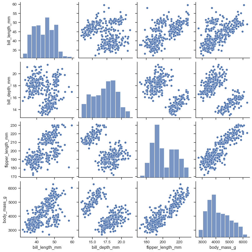
ref: seaborn.pairplot
カテゴリ変数ごとの傾向を見る#
1
| sns.FacetGrid(df, col="time", row="sex").map(sns.scatterplot, "total_bill", "tip")
|
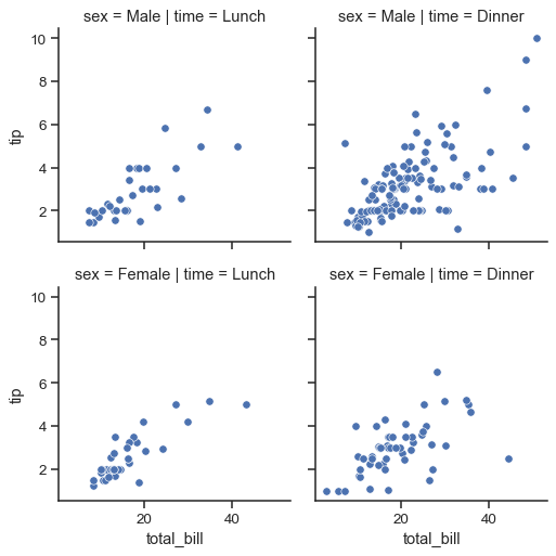
ref: seaborn.FacetGrid
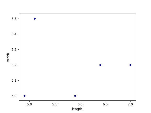
散布図#
1
| df.plot.scatter(x='length',y='width')
|
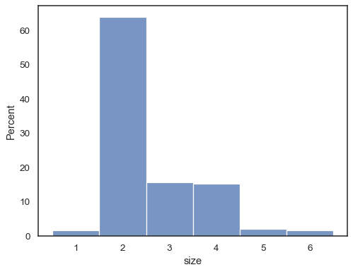
ヒストグラム#
1
| sns.histplot(data=df, x='Length', stat='percent')
|
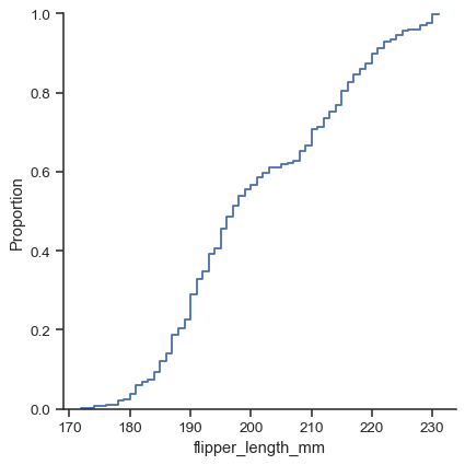
経験的累積分布関数#
1
| sns.distplot(data=df, x='Length', kind="ecdf")
|
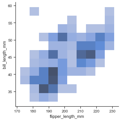
二変量プロット#
1
| sns.distplot(data=df, x='Width', y='Length')
|
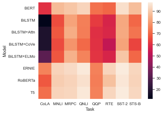
ヒートマップ#
統計的仮説検定#
二項検定#
2つのカテゴリに分類されたデータの比率が偏っているかどうかを検定する
A/BテストにおいてCVRに有意差があるかどうかなど
1
2
3
4
5
6
| from scipy import stats
x=500 #事象の発生回数
n=1000 #試行回数
a=0.5 #発生確率の帰無仮説
p = stats.binom_test(x, n, a)
print(p)
|
マンホイットニーのU検定#
2組の数値の集合が独立分布といえるかどうかを検定する
2つのクラスのテスト成績に有意差があるかどうかなど
1
2
3
| from scipy import stats
result = stats.mannwhitneyu(df['A'],df['B'],alternative='two-sided')
print(result.pvalue)
|
χ二乗検定(独立性検定)#
2つのカテゴリ変数が互いに独立であるかどうかを検定する
性別によって職業が左右されるかなど
1
2
3
4
| from scipy import stats
df=pd.crosstab(df['Job'],df['Sex'])
x2, p, dof, expected = stats.chi2_contingency(df)
print(p)
|
ref: クロス集計
分析モデル#
Cox比例ハザードモデル#
生存期間を予測する
1
2
3
4
5
6
7
| from lifelines import CoxPHFitter
cph = CoxPHFitter()
cph.fit(rossi, duration_col='lifetime', event_col='is_dead')
cph.print_summary()
cph.plot()
|
機械学習#
学習データの用意#
テストデータと教師データの分割#
1
2
3
4
5
| from sklearn.model_selection import train_test_split
X=df.drop(index='Target')
y=df['Target']
train_X, test_X, train_y, test_y = train_test_split(X,y)
|
クロスバリデーション#
1
2
3
4
5
6
7
8
| from sklearn.model_selection import cross_validate
clf = RandomForestClassifier()
X=df.drop(index='Target')
y=df['Target']
scores = cross_validate(clf, X, y, scoring=['accuracy','precision','recall','f1'], cv=5)
print(scores)
|
特徴量選択#
ロジスティック回帰の決定関数における特徴量の係数を表示する#
 1
 2
 3
 4
 5
 6
 7
 8
 9
10
11
12
13
| from sklearn.linear_model import LogisticRegression
logreg = LogisticRegression()
logreg.fit(X_train, y_train)
y_pred = logreg.predict(X_test)
print(logreg.score(X_train, y_train))
coeff_df = pd.DataFrame(train_df.columns.delete(0))
coeff_df.columns = ['Feature']
coeff_df["Correlation"] = pd.Series(logreg.coef_[0])
coeff_df.sort_values(by='Correlation', ascending=False)
|
| Feature | Correlation |
|---|
| 1 | Sex | 2.201527 |
| 5 | Title | 0.398234 |
| 2 | Age | 0.287163 |
| 4 | Embarked | 0.261762 |
| 6 | IsAlone | 0.129140 |
| 3 | Fare | -0.085150 |
| 7 | Age*Class | -0.311200 |
| 0 | Pclass | -0.749007 |
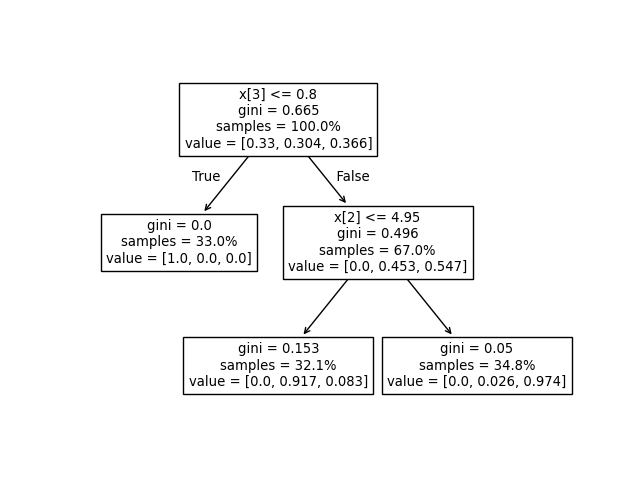
決定木モデルを可視化する#
 1
 2
 3
 4
 5
 6
 7
 8
 9
10
| from sklearn.tree import DecisionTreeClassifier,plot_tree
import matplotlib.pyplot as plt
clf = DecisionTreeClassifier()
clf.fit(X_train, y_train)
y_pred = clf.predict(X_test)
print(clf.score(X_train, y_train))
plot_tree(clf,max_depth=2)
plt.show()
|
モデル選択#
